Wave movement

Description

• Digital map of wave fields from L1-B level SAR images in fully automatic mode.
• Extraction of wave fields from SAR data
  • GWW function (of e-GEOS) based on models [ Hasselmann K. and S. Hasselmann , 1991, 1996] and on inversion techniques of [ Lyzenga DR, 2002].
  • Use of Level-1B SAR data from COSMO SkyMed , Radatsat-2, Sentinel-1.

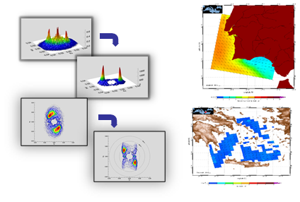
• Algorithm
  • SAR spectrum estimation
    • de-trending by Gaussian filtering,
    • identification and removal of the SAR IPR from detected (L1B) SAR data
    • removal of noise pedestal (speckle)
    • average of independent spectrum samples
  • SAR spectrum -> Sea spectrum
    • Hasselmann’s non-linear model inversion through cost function minimization
  • Spectral partitioning
    • identification of the partitions (in ω-θ-space)
    • estimation of significant wave height (Hs), wave-length and propagation directions for each identified wave system

Operating scenario

• Base knowledge

Technical specification

Requirement	Description
Spatial resolution	From 2 to 3 Km (depending on the SAR data used for estimation)
Coverage area	From 1600 to 60000 Km ^ 2 (depending on the SAR data used for estimation)
Geographic accuracy	5 m
Information Age	6 hours
Measurement uncertainty	Height: RMS <0.5m, Bias <0.1m Direction (for waves> 0.5m): RMS <30 °, Bias <10 ° Wavelength (for waves> 0.5m): RMS <50m, Bias <10m
Measurement / projection unit	Height and wavelength: meters Direction: degrees Projection: geographic ( lat / lon )
EO data in input	SAR data from COSMO- SkyMed , Radarsat-2 and Sentinel-1 (TOPS mode excluded)
Input data used	Optional: wind and wave forecasting models (WAM) from ECMWF and NOAA
Given for validation	data from buoy or altimeter in the test area
Algorithm method	Inversion of the Hasselmann model for the estimation of the sea surface spectrum starting from the estimation of the SAR spectrum. The inversion is based on the Lyzenga method which has proved effective in the Mediterranean area and does not necessarily require forecasting of input waves.
Format	NetCDF
Refresh rate	Given the availability of the SAR data on the area of ​​interest: 12 h

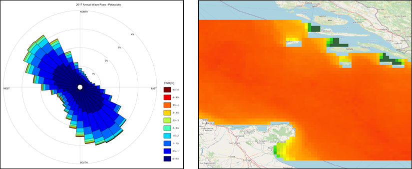
Statistical analysis

Requirement	Description
Spatial resolution	Less than 15 km.
Coverage area	Maximum extension of the AOI: 20000km 2
Geographic accuracy	Comparable with spatial resolution.
Information Age	Data not prior to 2008.
Measurement uncertainty	Dependent on the precision of the input data for which the following errors are expected: · Wave height ≤ 4m: Bias = -0.25m; RMS = 0.5m. Wave height> 4m: Bias = -0.5m; RMS = 0.6m. Wave direction: 45 degrees. (Confidence level: 90%)
Measurement / projection unit	Unit of measure · Return time: months. · Wind rose: meters for wave height and degrees for wave direction. Projection: Geographic-WGS84
EO data in input	–
Other input data used (not EO)	Data produced by a marine wave propagation model. The model outputs include the significant height of the wave with its associated direction.
Given for validation	In situ measurements or other EO data that will be identified during the project.
Format	GeoTIFF for the product “Return time”. png for the product “Wind rose”. Metadata: meet ISO 19115 standards, and specifications provided by the INSPIRE Directive 2007/2 / EC and the relevant Decree . n. 32 of 27/01/2010
Refresh rate	3 months

Example – wave movement

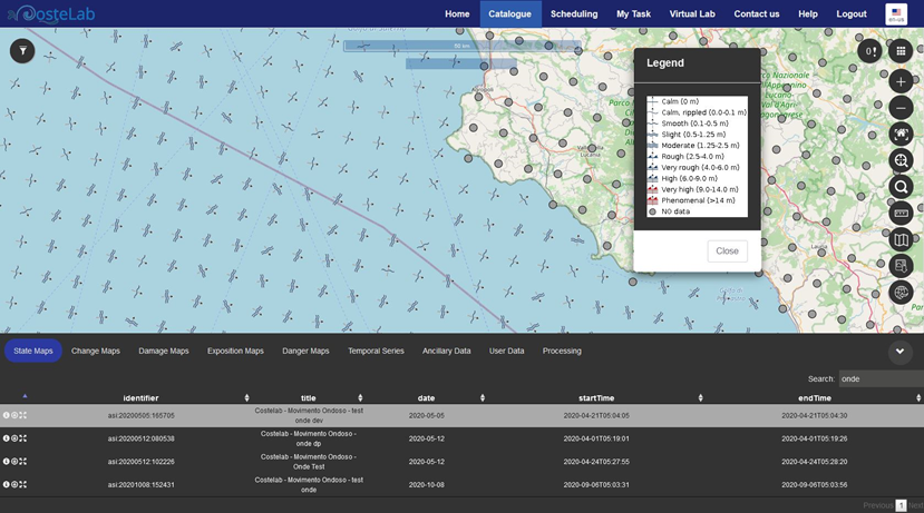
Examample – statistics on wave movement